Demystifying Network Infrastructure - From Basics to Data Centers for Developers

How does the network work? Having worked for over 10 years as an engineer, I still had many questions that I either did not understand or mistakenly believed. This happens because the network effectively abstracts all this complexity from us and significantly simplifies life. However, sometimes the lack of knowledge affected me; for instance, during an interview I was asked, “Which exact load balancer is needed here: Layer 3 or Layer 4?”, and I couldn’t answer precisely. Or, how is a packet transmitted over the network and how is this related to TCP/UDP? What is a connection? How are data centers set up from the inside, and how are they connected to the internet? How do BGP and anycast work, and where do they announce information about themselves? Recently, I decided to fill in these gaps and began to study network infrastructure, which became the basis for this article. This article will be useful for developers and SRE-engineers as our systems get bigger, deployed in multiple datacentres and we need a better understanding of the network in order to get better design results. I will try to add details that would be interesting to me as a developer. If you’re a network engineer, perhaps much of this is already familiar to you, so leave your comments and corrections.

Starting with the Basics

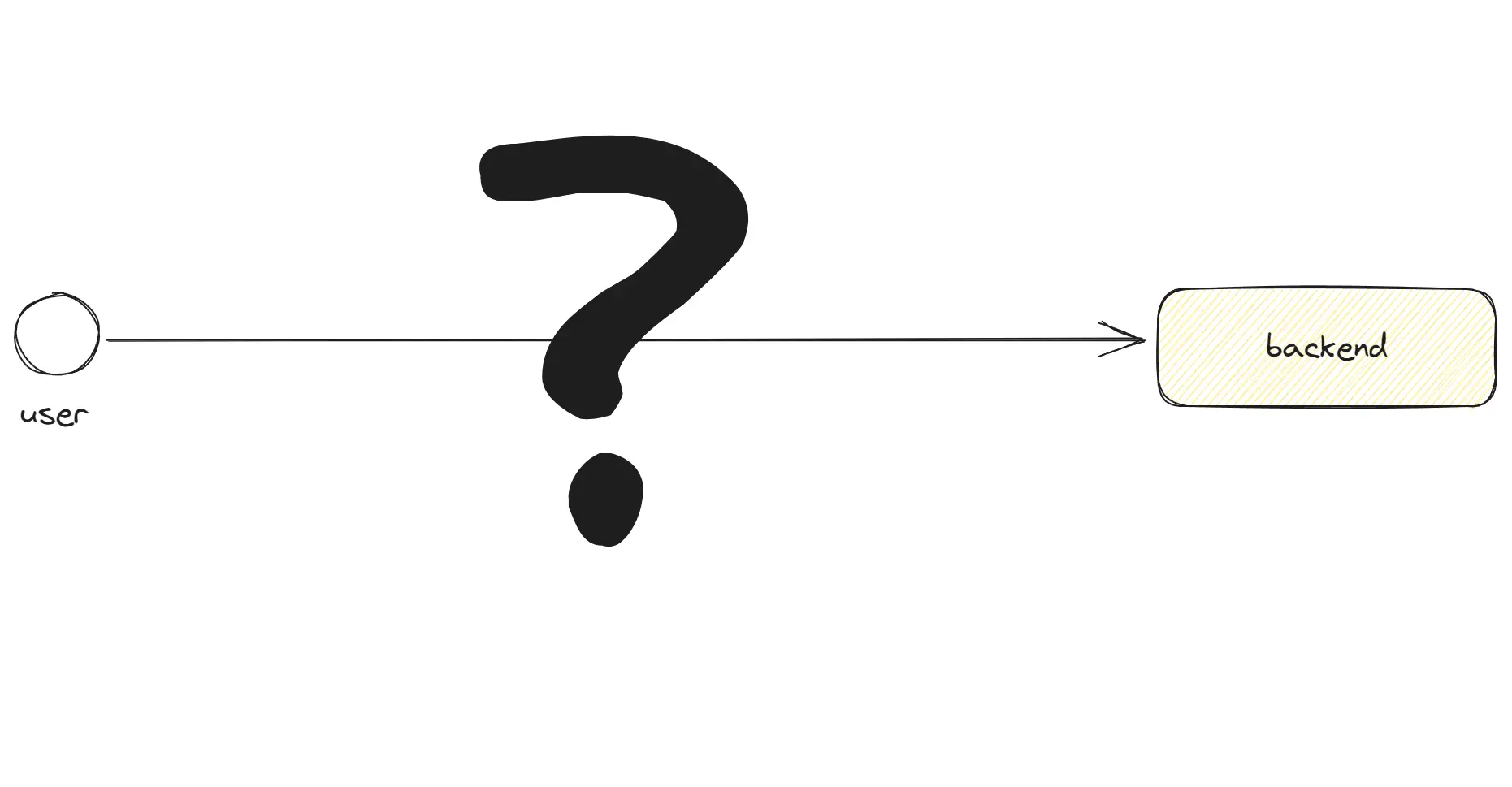
How does the network work? We can start with the basics:

• User — A user who wants to retrieve data from the backend.
• Backend — This is our application that delivers HTML pages.

But is everything really so simple in reality?

DNS - How to Determine Where to Connect?

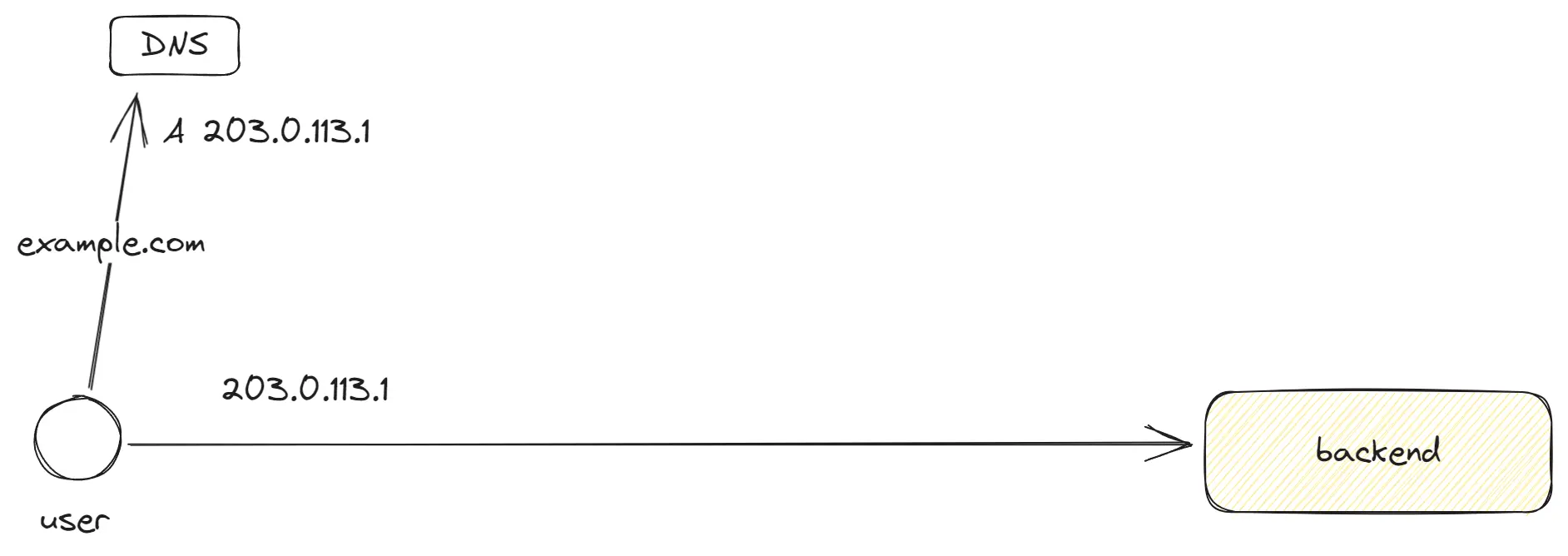
DNS (Domain Name System) — is a system that allows us to find IP addresses by domain names. It’s a kind of has map: we come with the domain example.com and get a list of IP addresses to connect to. Before making a request to a server, browsers and other systems first contact a DNS resolver and obtain an IP address that will be used for connection, as the entire internet operates on the basis of IP addresses.

In DNS it looks like this:

example.com. 300 IN A 203.0.113.1,
example.com. 300 IN A 203.0.114.1,
example.com. 300 IN A 203.0.115.1

Here is a list of A records that will be randomly chosen by the client when connecting. If one of the IP addresses doesn’t respond, the client switches to another. There are also AAAA records for IPv6.

GEO DNS allows you to link DNS records to regions. Thus, we can provide different IP addresses in different regions, for example, in Europe and America, distributing traffic and directing users to the nearest data center.

Scaling Traffic Handling with OSI Layers

If we have only one backend and we aim to handle a significant amount of traffic by adding another 20 backend applications, how can this be implemented?

OSI layers represent a virtual separation of the network structure into layers. This is done to simplify the description of systems and equipment, as well as to delineate responsibilities between the layers. The lower levels do not have information about the upper ones, and each subsequent level adds data to the previous ones. This structure can be visualized as a data stack: Stack = […Layer 7, …Layer 4, …Layer 3, …Layer 2].

Introducing OSI Layer 7 — Application Load Balancing

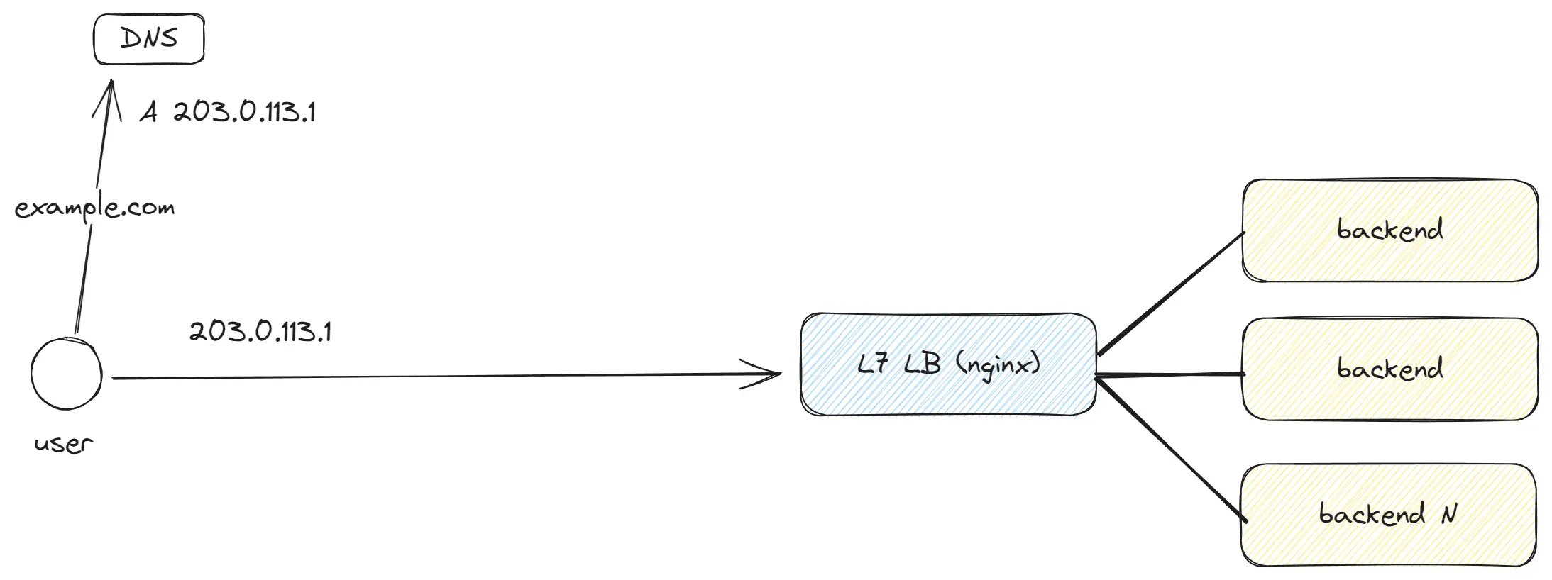
OSI Layer 7 is the topmost layer, where we work with requests containing a full set of data.

It’s important to note:

• There are different application layer protocols: HTTP 1, HTTP 2, HTTP 3, gRPC, WebSockets.
• HTTP 1, HTTP 2, and WebSockets operate over TCP, while HTTP 3 uses QUIC.
• It’s not mandatory to use L7 LB; you can choose L4 LB, which will proxy traffic directly to your backend application. However, in this case, the backend application will have to establish HTTPS connections on its own and won’t have the other features of L7 LB.
• L7 LB allows traffic balancing depending on paths, cookies, headers, performing data compression and decompression, caching, adding headers, http keepAlive and much more.

Here’s an example data format using the text format of HTTP 1.0: Request:

GET / HTTP/1.0
Host: example.com
User-Agent: Mozilla/5.0 (Windows NT 10.0; Win64; x64)
Accept: text/html,application/xhtml+xml,application/xml;q=0.9,image/webp,*/*;q=0.8

Response:

HTTP/1.0 200 OK
Content-Type: text/html; charset=UTF-8
Content-Length: 138
Date: Sat, 30 Oct 2021 17:00:00 GMT

<html>
<head>
<title>Example Domain</title>
</head>
</html>

Headers come first, followed by a separator, and then the data body. All of this is sent to Layer 4, where further processing occurs.

Introducing OSI Layer 4 - Transport Load Balancing

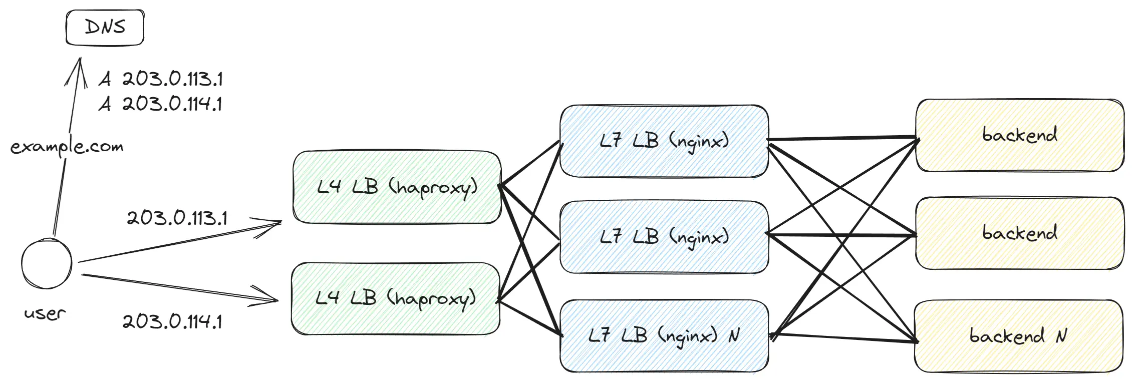
As we aim to process more traffic and the number of LBs begins to significantly increase, this creates an issue for DNS – we find ourselves listing dozens of IP addresses. Is there a more efficient way? As a solution, we introduce another level of abstraction by adding L4 LB, which will balance traffic between our L7 LBs. L4 LB operates faster and can handle more traffic since it is simpler in comparison to L7, and this allows us to continue scaling the L7 LB.

Layer 4 — Transport Layer, deals with TCP/UDP, and at this level, only the functions of the TCP/UDP transport protocol are available. We don’t have information about the path, request headers, and other details; we only know the port and IP address.

TCP

TCP (Transmission Control Protocol) is a protocol widely used on the internet. HTTP 1 and HTTP 2 are based on it. Inside TCP, the request is broken down into many Segment units of data, each up to 1460 bytes (20 bytes for headers). Here’s a data example (in reality, this is a byte array, not JSON):

{
  "source_port": 49562,
  "destination_port": 443,
  "sequence_number": 123456,
  "acknowledgment_number": 789012,
  "data_offset": 5,
  "flags": { SYN: 1, ACK: 0, ... },
  "window_size": 65535,
  "checksum": "0x1a2b3c4d",
  "data": "Encrypted (or plain) payload from higher layers..."
}

TCP requires establishing a connection between the client and the server. This is achieved in three stages, involving the sending of three packets:

1. Client -> Server: SYN - The client initiates the connection, indicating its ISN (initial sequence number).
2. Server -> Client: SYN, ACK - The server responds, providing its ISN and an ACK equal to the client’s ISN + 1 (accounting for the packet sent by the client).
3. Client -> Server: ACK - The client confirms its readiness to exchange data.

Thus, establishing a TCP connection requires three packets, and this can be problematic with significant delays (e.g., 300 ms) between the client and server. However, this is a TCP requirement from which we cannot escape, as the ISN is later used to determine the packet order. After creating the connection client and server have TCP keepAlive, which allows them to keep the connection open for a long time.

One of TCP’s main features is Reliability: it guarantees data delivery. If a packet isn’t delivered, it will be resent. However, as I mentioned earlier, one TCP Segment consists of 1460 bytes. Awaiting confirmation from the server for the delivery of each segment would take a vast amount of time. To solve this problem, TCP employs the Window Size mechanism, allowing a bunch of Segments to be sent and waiting for confirmation for the entire group.

By default, the Window Size is 65535 bytes, allowing 45 segments to be sent before receiving a confirmation. But even 65535 bytes isn’t that much. To accelerate data transfer in TCP, Congestion control algorithms are used, which can increase the Window Size depending on the quality of the channel between the client and server.

Optimization methods:

• Consider enabling TCP BBR for faster file transfer.
• Turn on TCP Window Scaling to increase the maximum Window Size to 1 GB.
• Enable TCP Fast Open to reduce the number of round trips when establishing a connection.

UDP

UDP (User Datagram Protocol) is a simple protocol that doesn’t offer many features available in TCP, but it’s lightweight. UDP breaks the request into Datagrams, each up to 1472 bytes in size (8 bytes in headers). Here’s a data example (in reality, it’s a byte array, not JSON):

{
  "source_port": 49562,
  "destination_port": 443,
  "length": 1472,
  "checksum": "0x1a2b3c4d",
  "data": "Encrypted (or plain) payload from higher layers..."
}

Unlike TCP, UDP doesn’t guarantee data delivery, so if guaranteed delivery is required, it must be implemented independently.

QUIC

QUIC (Quick UDP Internet Connections) is a new protocol based on UDP, with a similar Datagram format. For most servers, QUIC traffic is hard to distinguish from UDP. However, QUIC implements all the key features inherent to TCP and even surpasses it in some aspects. The primary reason for QUIC’s creation is that TCP is difficult to modify due to its widespread use across tens of thousands of servers, and significant changes are needed to improve content delivery in TCP. Therefore, QUIC was developed, which is built on top of UDP and adds new functionalities. QUIC is used in HTTP 3.

What can you read next? https://www.smashingmagazine.com/2021/08/http3-core-concepts-part1/

Introducing OSI Layer 3 - Network Load Balancing

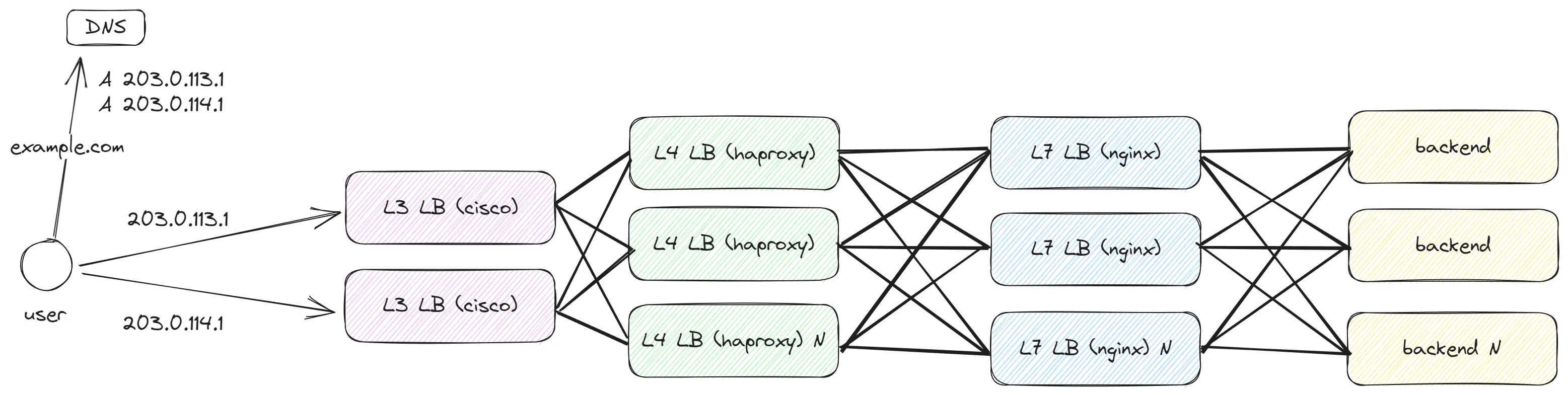
As we need to handle even more traffic and require an additional abstraction layer before L4 to scale the number of L4 LBs, the solution becomes the addition of L3 LB, which will balance traffic among our L4 LBs.

At Layer 3, Packet units are transmitted, which are then transmitted across the network. At this level, only the sourceIP and destinationIP are accessible. A packet has a size of up to 1500 bytes (20 bytes being headers) and follows this format:

{
  "sourceIP": "192.168.1.10",
  "destinationIP": "93.184.216.34",
  "TTL": 64,
  "protocol": "TCP" | "UDP",
  "data": "{ Entire L4 segment|datagram... }"
}

Key points:

• At this level, it generally doesn’t matter whether http2, http3, TCP, or UDP is used, as everything is simply packets being transferred from server to server.
• Packets go both from client to server and vice versa. For the client, a packet is created with the destinationIP set to the “target”, adding the client’s sourceIP. For the server, the packet is formed with the destinationIP set to the client’s sourceIP.
• During transmission, packets can take different paths. For example, one packet might go through Provider A, while another might go through Provider B. As a result, packets can arrive in a different order.
• Packets can be lost due to different paths, which can be overloaded. That’s why TCP uses Congestion control algorithms, allowing the resending of lost packets.
• There’s no concept of a session at this level. Packets go as they please, and the session in TCP is just an agreement between the client and server that doesn’t influence packet transmission in the network.

Optimization methods:

• Enable ECMP - this will allow the use of multiple paths for packet transmission.
• Enable Anycast - this allows using the same IP address in different parts of the world, reducing latency and increasing availability.

How is the network structured between the user and the server?

The modern internet consists of numerous cables transmitting data. There are limited cables, and client types vary: from a regular user wanting to watch YouTube to a massive data center with thousands of servers. Various network types, interconnected by cables, exist to connect all clients and transmit traffic to one another. Different levels pay each other for data transmission, hence the drive to optimize traffic at their level. A typical client connecting to the internet begins its operations with Tier 3 and subsequently utilizes all other levels.

ISPs and peering

Tier 3 (Local level)

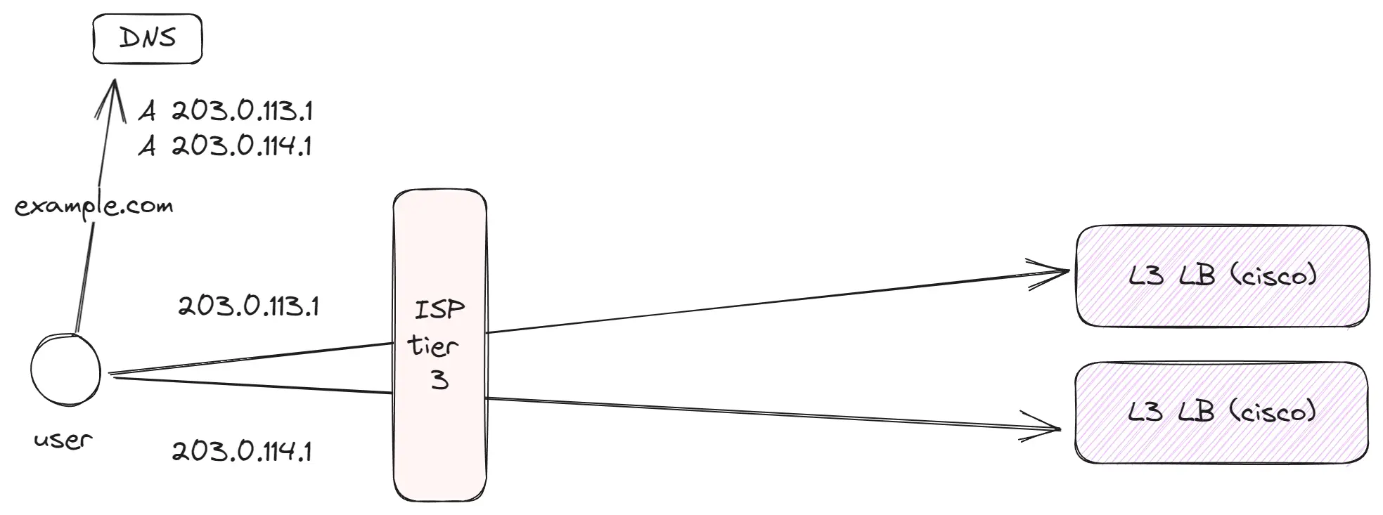
These are thousands of smaller providers in cities and regions that act as the first link for regular clients. Then, these providers purchase or use dedicated channels to more prominent Tier 2 providers, who in turn, transmit traffic to the global internet.

Key points:

• Within Tier 3, there are typically clients of one provider or a union of providers if peering is established between them.
• Regular users utilize Tier 3 for data access. For instance, I use such a network for internet at home.
• Even at this level, some companies generating substantial traffic (like YouTube or Netflix) place their caching equipment, helping to alleviate the provider’s network load and enhance the service quality.

Tier 2 (Regional level)

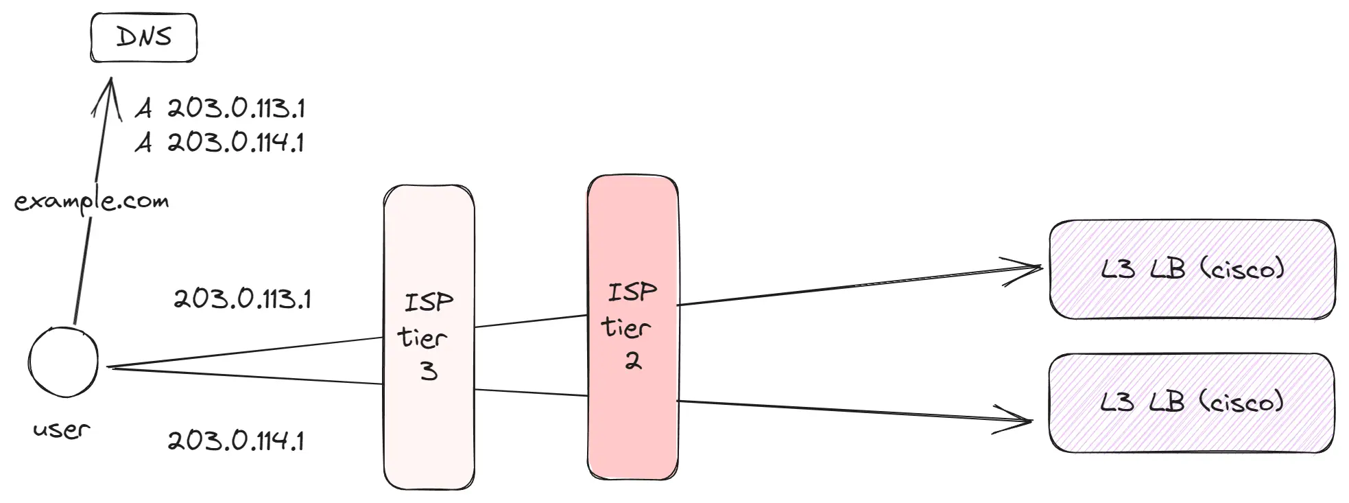
These are hundreds of large or regional providers servicing a vast number of clients. They focus on more local or regional traffic. Tier 2 providers connect with neighboring Tier 2 providers and utilize Tier 1 to access the global internet.

Key points:

• Companies such as Amazon, Google, and Facebook position their Edge servers at this level to be as close as possible to the end-users.

Tier 1 (Global level)

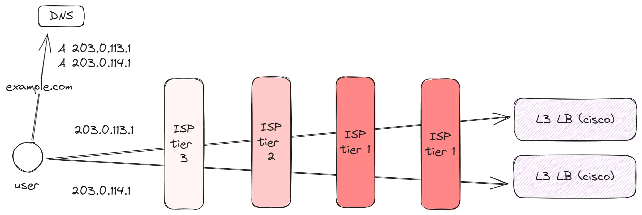
These are a few dozen global players controlling the primary communication channels between different geographic points – for example, between Europe and America or America and Asia. Thanks to them, while being in Europe, one can effortlessly visit a site hosted in Japan.

Key points:

• Tier 1 providers have vast channels connecting different parts of the world. For instance, there are channels linking Europe with America or America with Asia.
• Between distant regions, such as Europe and Asia, several different channels operate.
• Some requests might pass through multiple Tier 1 providers.

How does a user locate a server by IP address? (BGP, Anycast)

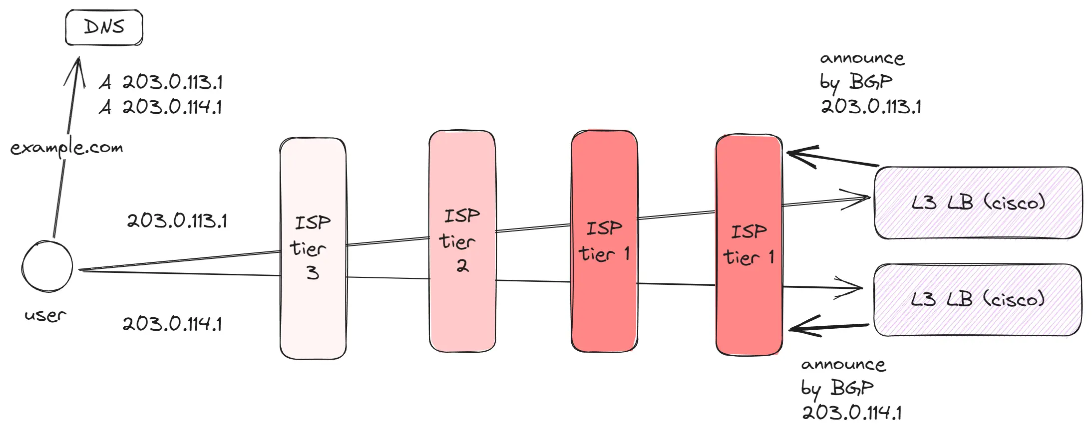
There are millions of IP addresses. So, how can a regular client connected to the internet determine where to direct requests based on an IP address?

• A server uses BGP to announce its IP address to the nearest Tier 1 or Tier 2 provider. BGP is a protocol that is adopted and used by all internet providers. It stores information about servers capable of handling traffic for specific IP addresses.
• Once our server communicates its IP address to a Tier 1 provider, this provider relays this information to all neighboring Tier 1 and Tier 2 providers, who in turn share it with Tier 3.
• When a user makes a request by IP address, it forwards the request to the Tier 3 level. Upon receiving the request, Tier 3 checks the routing table to determine which subsequent server announced this IP address and redirects the packet to it. This process continues until the request reaches the target server.

This mechanism allows for additional optimizations:

• Anycast enables the use of the same IP address in different parts of the world, reducing latency and improving availability. Thus, at the Tier 2 level, a server can be set up that will announce the same IP address. As a result, two servers capable of handling traffic from one IP address will appear on the internet. Nearby clients will connect to the nearest server, and traffic will be directed to it.

Edge Networks

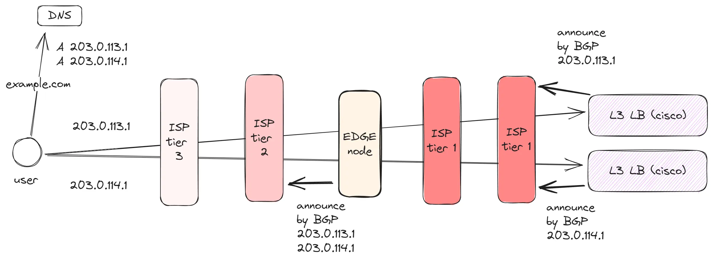
BGP and Anycast pave the way for the development of Edge networks, which are actively used by companies such as AWS, Cloudflare, and Google. There are a limited number of data centers, and hundreds of millions of users are at a distance from these data centers. However, we need these users to be able to quickly load data and have a fast connection.

To address this, space is rented in data centers at various geographic points, where companies place their equipment. Taking Google as an example: they have 39 data centers and 187 points where Edge equipment is installed. An Edge network contains:

• Proxy equipment, which announces IP addresses using Anycast. By announcing an IP address in different locations, users connect to the nearest server, reducing latency. Since the distance between the user and Edge equipment is shorter, there is less ping, resulting in faster TCP connections. Also, between Edge and the data center, quality/dedicated connections are established for data transfer.
• Caching equipment, which stores frequently requested data in the region, such as images, videos, JS files, and other assets. This reduces the strain on the channel to the data center and accelerates data loading for users.
• Edge Computing, some companies, like CloudFlare, have gone a step further and allow code to be executed on Edge equipment. This enables the creation of backend applications that are very close to users. Thus, even remote users receive data as quickly as those near the data center.

Data Center Networks

Now comes the most interesting part. In reality, data centers look different than I previously showed. Earlier diagrams more accurately depicted a packet’s journey in a simplified form, which is convenient when I draft design documents. However, in reality, data centers are configured to handle vast amounts of diverse traffic with low latency. I’ll be exploring based on the data centers used by the company Meta, which gives a detailed account of their DCs. Kudos to them for that. It’s worth noting that Meta has state-of-the-art data centers, and unfortunately, not everyone has the same.

Features of modern data centers include:

• Modular design: Data centers are built and designed as blocks, which can be easily added or removed. Each block contains all the necessary equipment with a well-thought-out network architecture. This simplifies the design and standardizes the equipment.
• Energy, bandwidth, and space requirements: Data centers are physical entities, so additional nuances arise. You can’t just add a bunch of servers if there isn’t sufficient energy, communication channels, and space.
• Huge speeds: Data centers operate hundreds of terabits of data per second. For instance, my home internet is only 0.5 gigabits per second, which is a thousand times less.
• Data centers are integrated into regions: Companies don’t just build a single DC. Instead, they form a region comprising 3 or more DCs, also called zones. These zones are located close to each other, have different energy sources and communication channels, and are interconnected with dedicated communication lines. This way, if one DC fails, the others can take over its workload, and users won’t notice a problem if the service was designed correctly.
• Focused on internal traffic: In today’s world, 80% or more of the data center traffic is internal and doesn’t go outside. This is because when a user request arrives at a service, we often need to access cache, databases, other services, and analytics. Minimal latency for internal requests is crucial.

Let’s delve into how a Zone is structured.

Rack

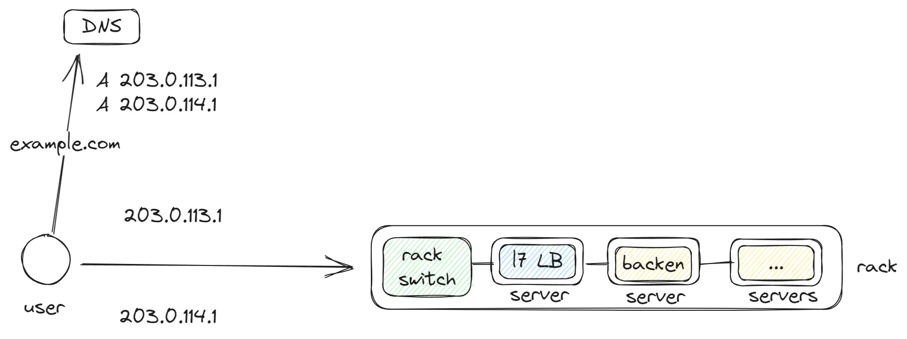
A Rack is the basic unit in a data center, to which many servers are connected. Inside these servers, containers (like Docker) run, and inside them are applications, L7 LB, databases. Each Rack is equipped with a rack switch to which the other servers are connected, handling all the traffic.

In a single data center or region, there can be thousands of such Racks.

Fabric switch

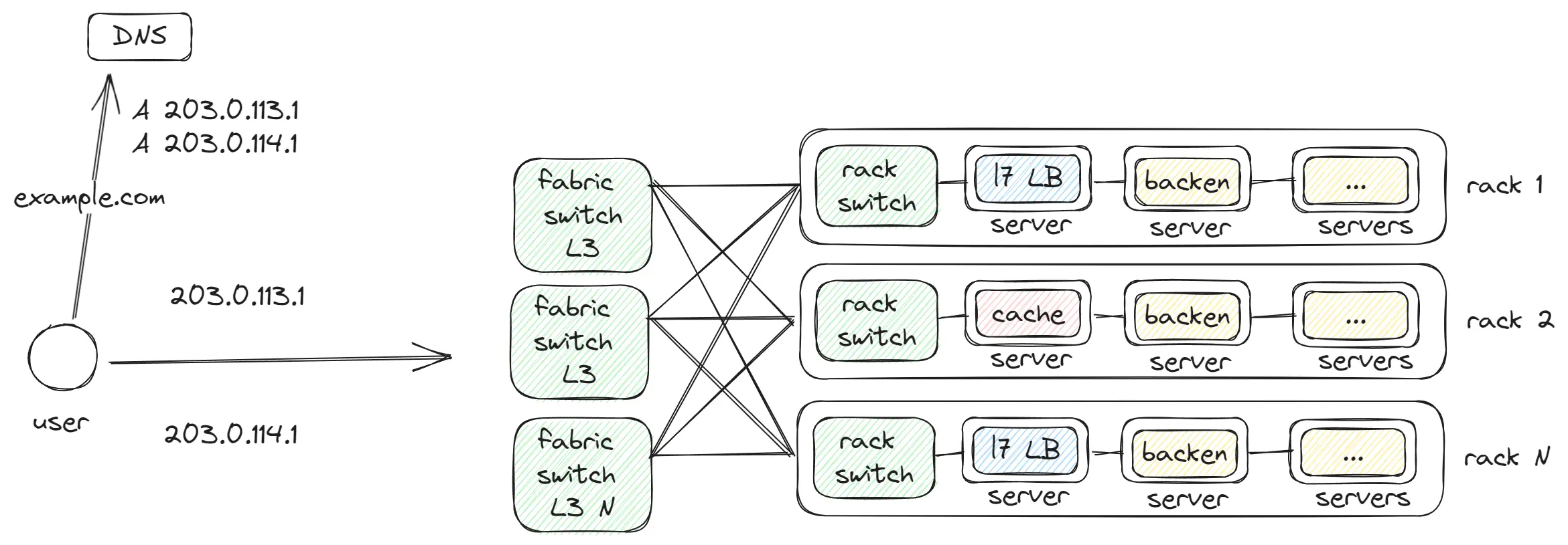
The Fabric switch is networking equipment that connects groups of rack switches. Our applications frequently exchange data, and these services are often on neighboring Racks. To achieve minimal latency, equipment connecting up to 128 Racks into one network is used. Thus, a request from Rack 1 can reach Rack 2 in a single hop.

But a fabric switch can connect up to 128 rack switches, requiring additional levels to interconnect the fabric switches.

Spine switch

Spine switch connects the fabric switch together, as we face a limitation on the number of available ports on the Fabric switch. This is a somewhat similar problem to what we had before with L7/L4/L3.

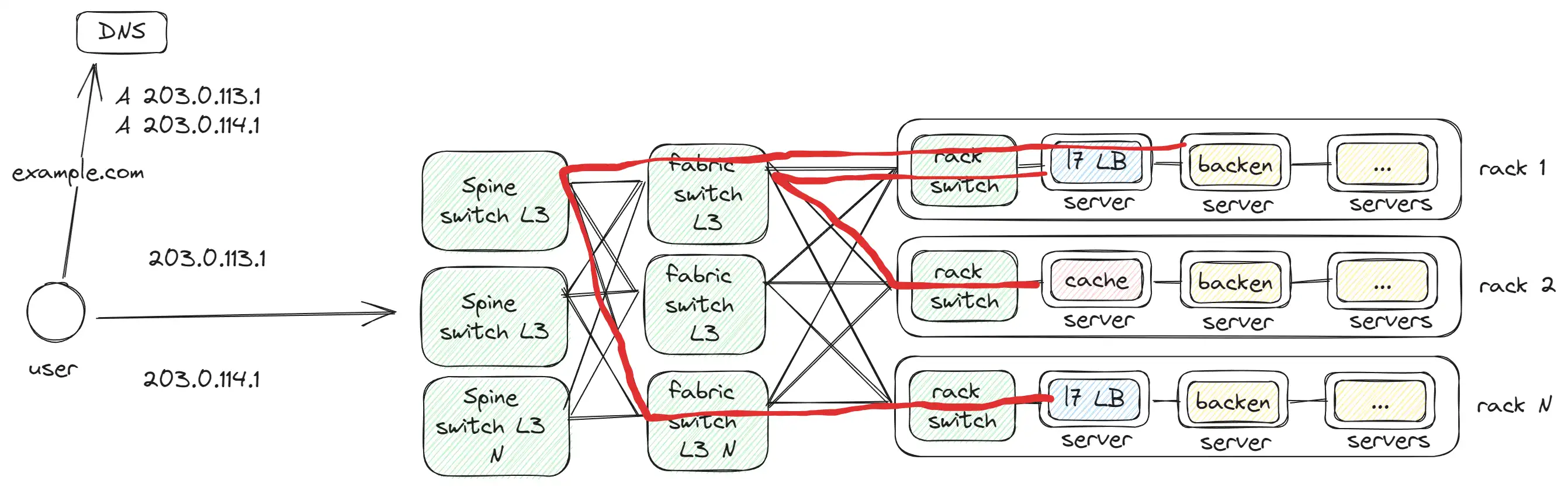
The red line illustrates how communication occurs:

• Between 2 Rack in 1 hop, as they are connected to the same Fabric switch.
• Between 2 Rack in 3 hops, since they are connected to different Spine switches.

Fabric aggregator and Zone

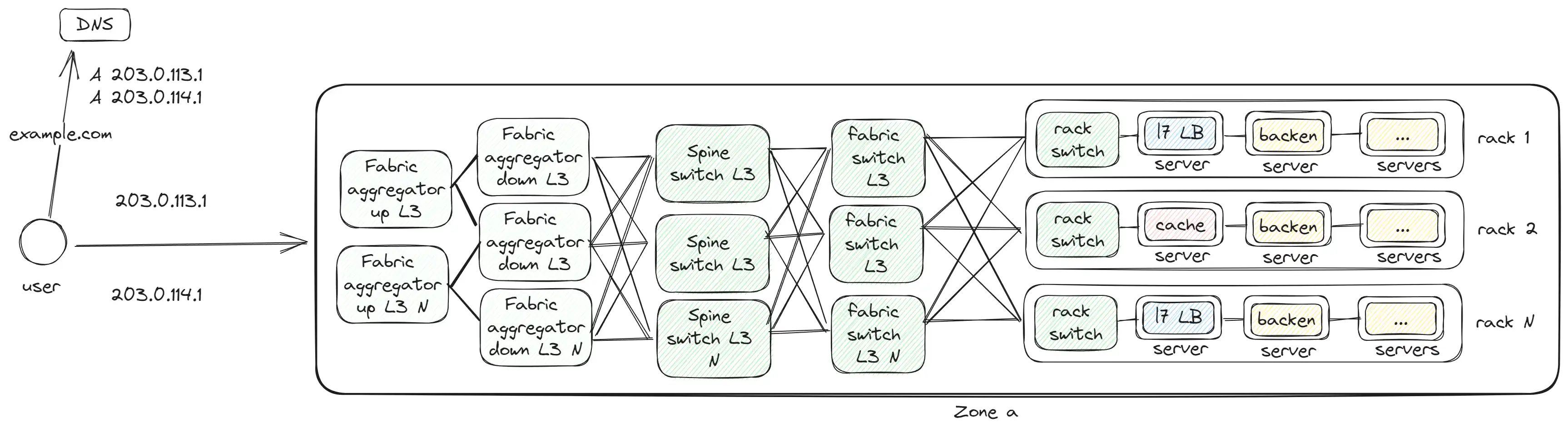
With the addition of the Fabric aggregator, a full-fledged zone or data center forms. This represents the level of a large building.

The Fabric aggregator connects different zones and handles external traffic. Considering the large volume of internal traffic, different equipment is needed for external and internal traffic. Therefore, Meta divided it into two levels:

• Fabric aggregator down — handles internal traffic between zones and is connected to every Spine switch of other zones.
• Fabric aggregator up — handles external traffic coming in or going out.

Region

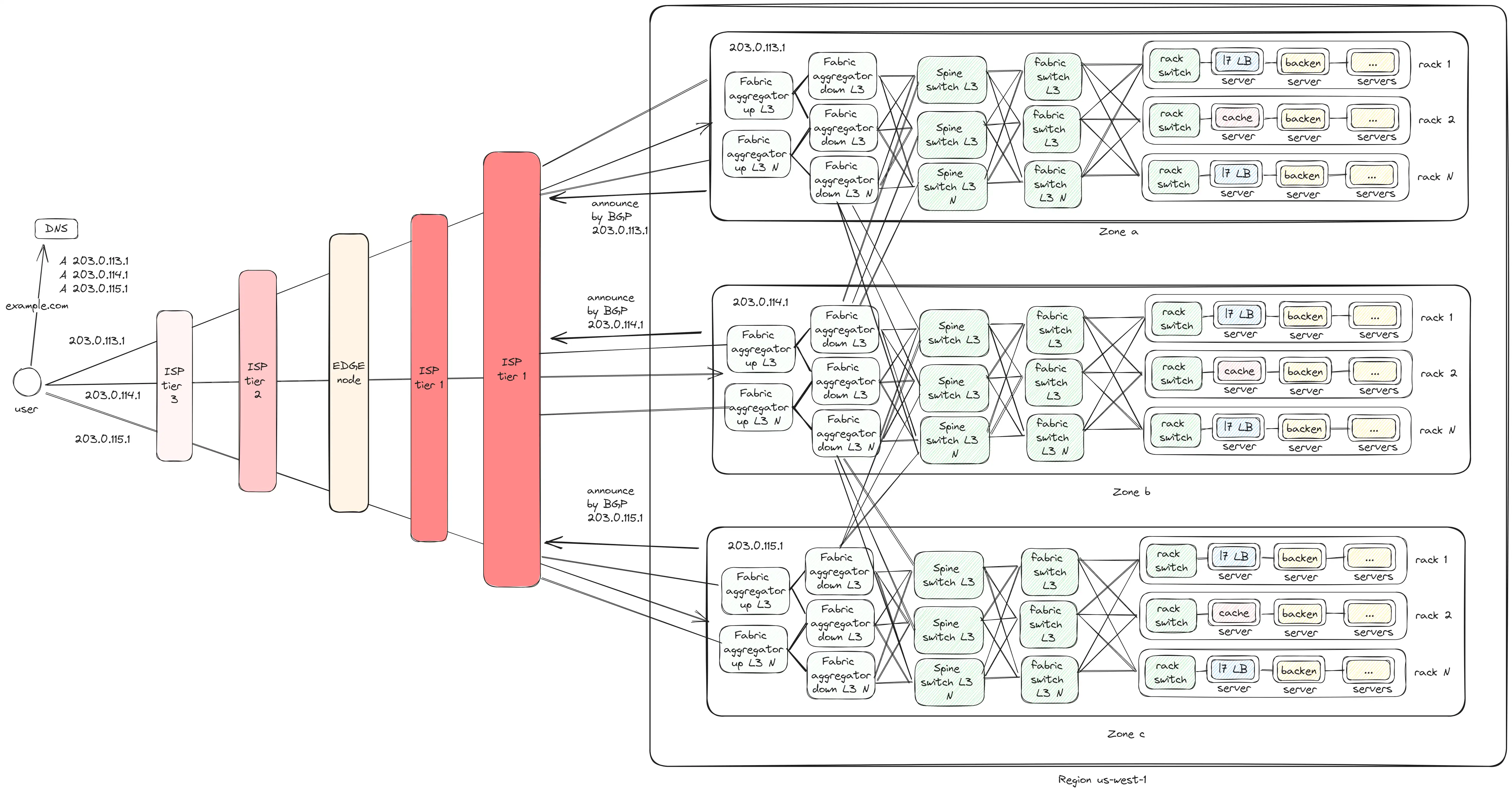
In the end, we arrive at the final version where we have 3 regions:

• All regions are interconnected through the Fabric aggregator down.
• Regions are connected to ISPs via the Fabric aggregator up.
• Regions announce themselves through BGP so users can find them by IP address.
• Requests within a single Zone are executed with a maximum of 6 hops; between Zones — 8 hops.

Additional Points

Future Scalability

All this can be scaled, resulting in 6 zones in one region, which would look truly epic. 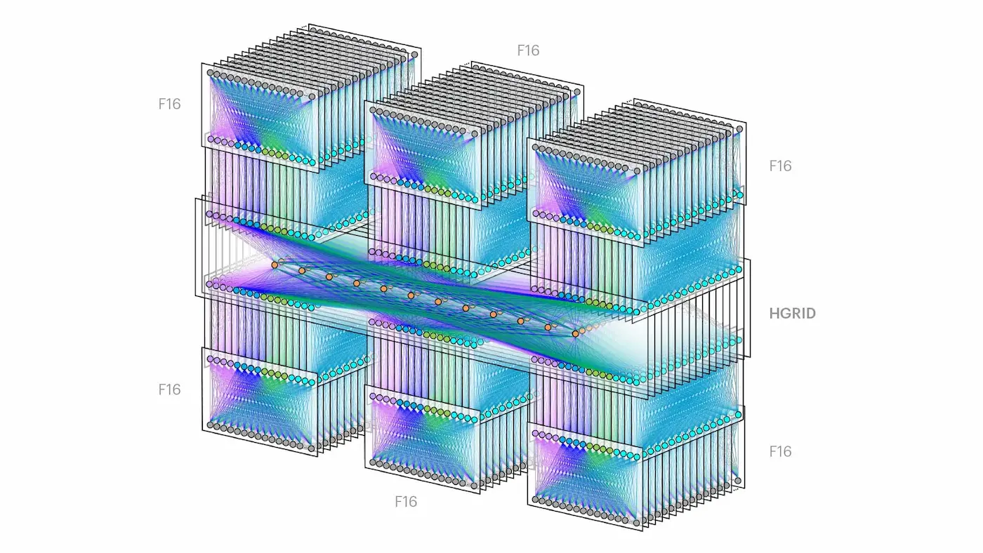It might seem complicated at first glance. However, if you break it down, each “tower” is a Zone from my diagram, and in the middle is the Fabric aggregator layer. I still wonder: how many cables would be required to connect all this?

Application Development Recommendations

I recommend planning the architecture and infrastructure of the project, considering the use of local traffic within the Zone, synchronizing data only between zones and regions. This way, you can achieve minimal latency and cost, as traffic between zones and especially between regions is chargeable.

Why have 3+ Zones in Region, and not 2 or 1?

It all boils down to redundancy. Data centers, infrastructure, and systems must be designed with the possibility of part of the system failing. Numerous reasons can cause such a failure: internet disruption, power outage, or a fire. Considering this risk, a backup system is essential. Take, for example, a need to handle 10,000 rps:

• If we have 2 DCs/Zones in one region, each needs resources to handle 10,000 RPS. If 1 DC fails, the other will have the resources to manage. This means an extra 10,000 rps will be idly reserved.
• With 3 DCs in one region, each only needs resources for 5,000 RPS, reducing the reserve to 5,000 rps.

Thus, having at least 3 Regions/DCs in one region is much more economical in terms of resources.

Conclusion

Networking is a vast and fascinating subject. I’ve covered only part of the issues, without delving into topics like virtual networks, dividing the network into external and internal, and many others. Thank you for your time. If you find inaccuracies, mistakes, or have something to add, please comment. I’d be happy to discuss.

Sources

• https://research.google/pubs/pub44824/
• https://cloud.google.com/load-balancing/docs/application-load-balancer
• https://www.nextplatform.com/2021/11/11/getting-meta-abstracting-and-multisourcing-the-network-like-an-fboss/
• https://www.youtube.com/watch?v=rRxGJbu8nqs
• https://engineering.fb.com/2019/03/14/data-center-engineering/f16-minipack/
• https://cloud.google.com/about/locations#lightbox-regions-map
• https://cloud.google.com/compute/docs/ip-addresses#reservedaddress